Synthetic Trees
When testing and using simulation models we often need to use synthetic data. This might be because we want to examine the effects of different initial conditions on our model output, or simply because we have insufficient data to examine a system at the scale we would like to. The ecological-economic modelling project I'm currently working on is in both these situations, and over the last week or two I've been working on generating synthetic tree-level data so that we can initialize our model of forest stand change for testing and scenario development. Here's a brief overview of how I've approached the task of producing a 'treelist generator' from the empirical data we have for over 60,000 trees in Northern Hardwood stands across Upper Michigan.
One of the key measures we can use to characterise forest stands is basal area (BA). We can assume that for each stand we generate a treelist for there is some 'target BA' that we are aiming to produce. As well as hitting a target BA, we also need to make sure that the tree diameter-at-breast-height (DBH) size-class distribution and species composition are representative of the stands in our empirical data. Therefore, our the first step is to look at the diameter size-class distribution of the stands we want to emulate. We can do this by plotting histograms of the frequency of trees of different diameter for each stand. In the empirical data we see two characteristic distributions (Fig 1).
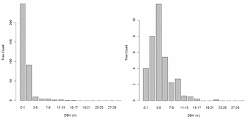
Fig 1. Example stand tree count histograms
The distribution on the left has very many more trees in the smaller size classes as a result of stands self-thinning (as larger trees compete for finite resources). The second distribution, in which the smallest size classes are under-represented and larger size classes have relatively more trees, does not fit so well with the theoretical, self-thinning DBH size-class distribution. Stands with a distribution like this have probably been influenced by other factors (for example deer browse on the smaller trees). However, it turns out that both these DBH size-class distributions can be pretty well described by the gamma probability distribution (Fig 2).
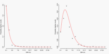
Fig 2. Example stand gamma probability distributions for data in Fig 1
The gamma distribution has two parameters, a shape parameter we will call alpha and a scale parameter we will call beta. Interestingly, in the stands I examined (dominated by Sugar Maple and Ironwood) there are two different linear relationships between the parameters. The relationship between alpha and beta for 80% of stands represents the 'self-thinning' distribution, and the other 20% represent distributions in which small DBH classes are under-represented. We use these relationships - along with the fact that the range of values of alpha for all stands has a log-normal distribution - to generate characteristic DBH size-class distributions;
So now for each stand we have a target basal area, and parameters for the DBH size class distribution. The next step is to add trees to the stand with diameters specified by the probability distribution. Each time we add a tree, basal area is added to the stand. The basal area for a tree is calculated by:
TreeBA = TreeDensity * (0.005454* diameter2)
[Tree density can be calculated for each tree because we know the sampling strategy used to collect empirical data on our timber cruise, whether on a fixed area plot, n-tree or with a prism].
Once we get within 1% of our target BA we stop adding trees to the stand [we'll satisfy ourselves with a 1% accuracy because the size of tree that we allocate each time is sampled from a probability distribution and so we it is unlikely we will be able to hit our target exactly]. The trees in our (synthetic) stand should now (theoretically) have the appropriate DBH size-class distribution and basal area.
With a number of trees in now in our synthetic stand, each with a DBH value, the next step is to assign each tree to a species so that the stand has a representative species composition. For now, the two species we are primarily interested in are Sugar Maple and Ironwood. However, we will also allow trees in our stands to be Red Maple, White Ash, Black Cherry or 'other' (these are the next most common species in stands dominated by Sugar Maple and Ironwood). First we estimate the proportion of the trees in each species. In stands with Sugar Maple and Ironwood deer selectively browse Sugar Maple, allowing Ironwood a competitive advantage. Correspondingly, in the empirical data we observe a strong linear and inverse relationship between the abundance of Sugar Maple and Ironwood (Fig 3).
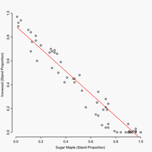
Fig 3. Relationship between stand Sugar Maple and Ironwood abundance
To assign species proportions we first estimate the proportion of Sugar Maple from the empirical data. Next, using the strong inverse relationship above we estimate the corresponding proportion of Ironwood (sampled using normal distribution with mean and standard deviation from from Bayesian linear regression). The remaining species proportions are assigned according to the frequency of their presence in the empirical data.
Now we use these proportions to assign a species to individual trees. Because physiology varies between species, the probability that a tree is of a given size also varies between species. For example, Ironwood very seldom reach DBH greater than 25 cm and the vast majority (almost 99% in our data) are smaller than 7.6 cm (3 inches) in diameter. Consequently, first we assign the appropriate number Ironwood to trees according to their empirical size-class distribution, before then assigning all other trees to the remaining species (using a uniform distribution).
The final step in generating our treelist is to assign each tree a height and a canopy ratio. We do this using empirical relationships between diameter and height for each species that are available in the literature (e.g. Pacala et al. 1994). And we're done!
In the model I'm developing, these stands can be assigned a spatial location either using a pre-existing empirical map or using a synthetic land cover map with known characteristics (generated for example using the modified random clusters method, as the SIMMAP 2.0 software does). In either case we can now run the model multiple times to investigate the dynamics and consequences of different initial conditions. More on that in the future.
One of the key measures we can use to characterise forest stands is basal area (BA). We can assume that for each stand we generate a treelist for there is some 'target BA' that we are aiming to produce. As well as hitting a target BA, we also need to make sure that the tree diameter-at-breast-height (DBH) size-class distribution and species composition are representative of the stands in our empirical data. Therefore, our the first step is to look at the diameter size-class distribution of the stands we want to emulate. We can do this by plotting histograms of the frequency of trees of different diameter for each stand. In the empirical data we see two characteristic distributions (Fig 1).

The distribution on the left has very many more trees in the smaller size classes as a result of stands self-thinning (as larger trees compete for finite resources). The second distribution, in which the smallest size classes are under-represented and larger size classes have relatively more trees, does not fit so well with the theoretical, self-thinning DBH size-class distribution. Stands with a distribution like this have probably been influenced by other factors (for example deer browse on the smaller trees). However, it turns out that both these DBH size-class distributions can be pretty well described by the gamma probability distribution (Fig 2).

The gamma distribution has two parameters, a shape parameter we will call alpha and a scale parameter we will call beta. Interestingly, in the stands I examined (dominated by Sugar Maple and Ironwood) there are two different linear relationships between the parameters. The relationship between alpha and beta for 80% of stands represents the 'self-thinning' distribution, and the other 20% represent distributions in which small DBH classes are under-represented. We use these relationships - along with the fact that the range of values of alpha for all stands has a log-normal distribution - to generate characteristic DBH size-class distributions;
- sample a value of alpha from a normal distribution (subsequently reconvert using 10alpha),
- for the two different relationships use Bayesian linear regression to find mean and 95% credible intervals for the slope and intercept of a regression line between alpha and beta,
- use the value of alpha with the regression parameters to produce a value of beta.
So now for each stand we have a target basal area, and parameters for the DBH size class distribution. The next step is to add trees to the stand with diameters specified by the probability distribution. Each time we add a tree, basal area is added to the stand. The basal area for a tree is calculated by:
[Tree density can be calculated for each tree because we know the sampling strategy used to collect empirical data on our timber cruise, whether on a fixed area plot, n-tree or with a prism].
Once we get within 1% of our target BA we stop adding trees to the stand [we'll satisfy ourselves with a 1% accuracy because the size of tree that we allocate each time is sampled from a probability distribution and so we it is unlikely we will be able to hit our target exactly]. The trees in our (synthetic) stand should now (theoretically) have the appropriate DBH size-class distribution and basal area.
With a number of trees in now in our synthetic stand, each with a DBH value, the next step is to assign each tree to a species so that the stand has a representative species composition. For now, the two species we are primarily interested in are Sugar Maple and Ironwood. However, we will also allow trees in our stands to be Red Maple, White Ash, Black Cherry or 'other' (these are the next most common species in stands dominated by Sugar Maple and Ironwood). First we estimate the proportion of the trees in each species. In stands with Sugar Maple and Ironwood deer selectively browse Sugar Maple, allowing Ironwood a competitive advantage. Correspondingly, in the empirical data we observe a strong linear and inverse relationship between the abundance of Sugar Maple and Ironwood (Fig 3).

To assign species proportions we first estimate the proportion of Sugar Maple from the empirical data. Next, using the strong inverse relationship above we estimate the corresponding proportion of Ironwood (sampled using normal distribution with mean and standard deviation from from Bayesian linear regression). The remaining species proportions are assigned according to the frequency of their presence in the empirical data.
Now we use these proportions to assign a species to individual trees. Because physiology varies between species, the probability that a tree is of a given size also varies between species. For example, Ironwood very seldom reach DBH greater than 25 cm and the vast majority (almost 99% in our data) are smaller than 7.6 cm (3 inches) in diameter. Consequently, first we assign the appropriate number Ironwood to trees according to their empirical size-class distribution, before then assigning all other trees to the remaining species (using a uniform distribution).
The final step in generating our treelist is to assign each tree a height and a canopy ratio. We do this using empirical relationships between diameter and height for each species that are available in the literature (e.g. Pacala et al. 1994). And we're done!
In the model I'm developing, these stands can be assigned a spatial location either using a pre-existing empirical map or using a synthetic land cover map with known characteristics (generated for example using the modified random clusters method, as the SIMMAP 2.0 software does). In either case we can now run the model multiple times to investigate the dynamics and consequences of different initial conditions. More on that in the future.
Labels: Forests, MichiganUP, Modelling, Statistical

This work by James D.A. Millington is licensed under a Creative Commons Attribution-Noncommercial-Share Alike 3.0 United States License.


0 Comments:
Post a Comment
<< Home